Lecture 11: Equipartition of energy

Note

It is probable that in the long and honorable history of the Royal Society no mistake more disastrous in its actual consequences for the progress of science and the reputation of British science than the rejection of Waterston’s papers was ever made. [Meunier’s note: Waterston was the first to suggest that energy was equally distributed along all degrees of freedom in a system. His 1845 manuscript was rejected and ridiculed] – J.S. Haldane

Warning

This lecture corresponds to Chapter 19 of the textbook.

Summary

Attention

With the following chapters, we go head-first in the big pool of statistical mechanics! This is where students usually start to say “Ah! It makes sense now”. However, before getting there, we will need to do some work (punt: let’s stay positive) !

In this specific chapter, we will answer one important question: What happens if the system can exchange energy with its surroundings? Specifically, we will look at the regime of relatively high-temperature. At the end of this summary, we will highlight the conditions of applicability of the central theme treated here.

The starting point is a straightforward one: many “energy” terms in physics are some quadratic forms of a variable. For instance, the kinetic energy of a particle:

$E_{\rm KE }=\frac{1}{2} m v^{2},$

and the potential energy of a pendulum (small oscillations):

$E_{\rm PE }=\frac{1}{2} k x^{2}.$

See the blue box below to realize that in first approximation, the energy of most problems can be expressed as a sum of quadratic terms.

If a system can absorb energy because it is in contact with a reservoir held at temperature $T$ , where does the energy get stored?

We answer this by calculating the expectation value of the energy, using Boltzmann’s distribution. For a generic energy term of the form $E=\alpha x^2$ , we have:

$\expval{E}=\frac{\int_{-\infty}^{\infty} \alpha x^{2} e ^{-\beta \alpha x^{2}} d x}{\int_{-\infty}^{\infty} e ^{-\beta \alpha x^{2}} d x}=\frac{1}{2} k_{ B } T.$

This is the central result of this chapter: the expectation value of the energy is $1/2 k_B T$ regardless of the value of $\alpha$ ! In other words, each quadratic term will contribute an energy of $1/2 k_B T$ per degree of freedom. This is called the “qquipartition theorem”: each degree of freedom (expressed as a separate quadratic term in the energy function) contributes exactly the same energy.

Examples:

Translation motion of a monatomic gas molecule:

$\expval{E}=\frac{3}{2} k_{ B } T$

(3 degrees of translational motions).
Rotational motion in a diatomic gas:

$\expval{E}=\frac{5}{2} k_{ B } T$

(3 translations and 2 rotations)
Vibrational motion in a diatomic gas:

$\expval{E}=\frac{7}{2} k_{ B } T$

3 translations, 2 rotations, and two degrees of freedom due to the vibrations:

$E=\frac{1}{2} m v_{x}^{2}+\frac{1}{2} m v_{y}^{2}+\frac{1}{2} m v_{z}^{2}+\frac{L_{1}^{2}}{2 I_{1}}+\frac{L_{2}^{2}}{2 I_{2}}+\frac{1}{2} \mu\left(\dot{ r }_{1}-\dot{ r }_{2}\right)^{2}+\frac{1}{2} k\left( r _{1}- r _{2}\right)^{2}$

Note

Quadratic approximation

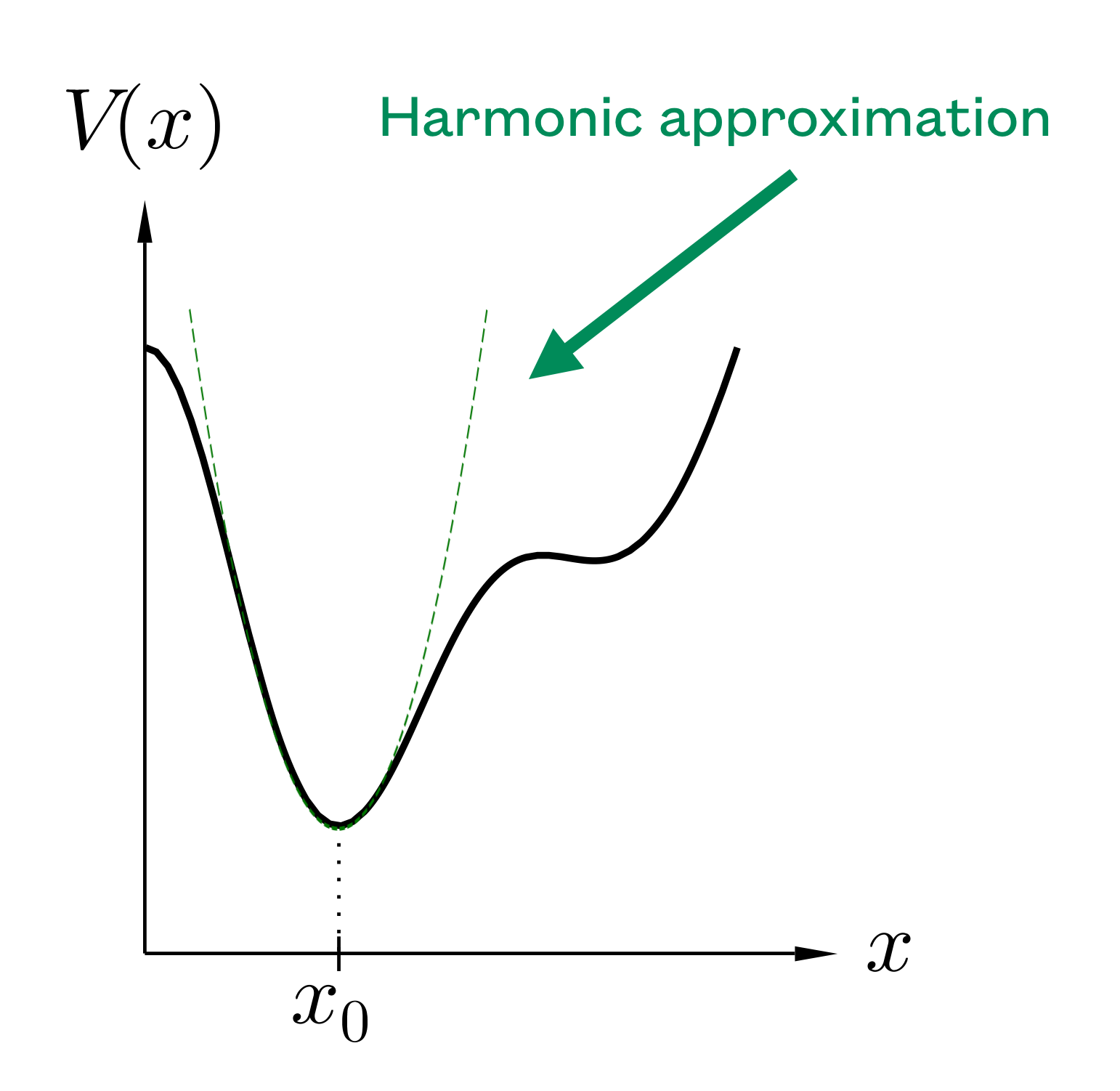
We know that the kinetic energy and the potential energy of a pendulum (small oscillations) are quadratic functions of the velocity and position, respectively. It appears that most problems can be expressed as a sum of quadratic terms. This comes from the simple observation of the Taylor’s series of an energy function around a minimum:

$V(x)=V\left(x_{0}\right)+\left(\frac{\partial V}{\partial x}\right)_{x_{0}}\left(x-x_{0}\right)+\frac{1}{2}\left(\frac{\partial^{2} V}{\partial x^{2}}\right)_{x_{0}}\left(x-x_{0}\right)^{2}+\cdots$

The second term on the right hand-side is zero at the minimum of the potential. It appears that, up to a reference energy shift, most potential functions are quadratic for small enough excursions away from the minimum (in that case we can ignore the higher terms). In contrast, we expect this approximation to break down at very high temperature, since the displacements become too large to ignore the high order terms.

Warning

Limitations of the equipartition theorem

The equipartition theorem is based on the fact that an integral such as the one shown above can be performed with a continuous variable. However, this is not compatible with quantum mechanics as it establishes that certainly quantities are quantized. Consequently: The equipartition theorem is generally valid only at high temperature, so that the thermal energy is larger than the energy gap between quantized energy levels.
At very high-temperature, the quadratic approximation described in the blue box above is not longer valid and the equipartition theorem no longer applies.

Key Definitions

Note

Dulong-Petit equation:: The DP equation establishes that the heat capacity of a solid at high temperature is exactly $3R$ . This is a direct consequence of the equipartition theorem. It is not valid at low temperature since quantum mechanical effects are prominent in that case.
Anharmonicity:: Anharmonicity describes a system that cannot be described with a quadratic (i.e., harmonic) term. This is also called the “non-linear regime”. It is more pronounced at high temperature.

A full list of terms, including the ones provided here, can be found in the Index.

Learning Material

Copy of Slides

The slides for Lecture 11 are available in pdf format here: pdf

Screencast

Test your knowledge

The equipartition theorem states that:
1. If a system in contact with a heat reservoir at temperature $T$ has $n$ modes, its average energy is $n \times k_BT/2$ , for all systems.
2. If a system in contact with a heat reservoir at temperature $T$ has $n$ modes, its average energy is $n \times k_BT/2$ , only if the modes are quadratic functions.
Consider a monatomic gas moving in a three-dimensional space.
1. The average energy is $3/2k_BT$ so long as the molecules of gas move freely.
2. The average energy is $3/2k_BT$ regardless on whether the molecules are subject to an external potential or not.
Consider a diatomic gas moving freely in a three-dimensional space. What can you tell about its average energy?
1. The average energy is $5/2k_BT$ and does not depend on the mass of the molecules.
2. The average energy is $5/2k_BT$ so long as the energy is expressed in Joule/Kg (this is known as the gravimetric energy.)
3. The average energy is $7/2k_BT$ and does not depend on the mass of the molecules.
4. The average energy is $7/2k_BT$ so long as the energy is expressed in Joule/Kg (this is known as the gravimetric energy.)
It is safe to say that if the equipartition theorem is valid at a certain temperature, it is also valid at low and high temperature.
1. True, the equipartition theorem is valid so long as the contributions to the energy are quadratic functions.
2. False, the equipartition theorem becomes increasingly incorrect at low temperature when the quantum mechanical nature of physics (such as the granularity of energy) becomes more and more apparent. It remains, however, correct at high temperature.
3. False, the equipartition theorem becomes increasingly incorrect at low temperature when the quantum mechanical nature of physics (such as the granularity of energy) becomes more and more apparent. It is becomes incorrect at high temperature since the particles tend to explore locations where the potential is no longer a sum of quadratic functions.

Hint

Find the answer keys on this page: Answers to selected test your knowledge questions. Don’t cheat! Try solving the problems on your own first!

Homework Assignment

Solve the following problems from the textbook: