Lecture 16: Phonons

Note

If you want to find the secrets of the universe, think in terms of energy, frequency and vibration. – Nikola Tesla

Warning

This lecture corresponds to Chapter 24 of the textbook.

Summary

Attention

In the previous lecture (Lecture 15: Photons) we focused on photons, which is one type of particles we investigated using what we learned regarding “a gas of particles”. This has been the recurring subject of most of our course so far. In this chapter, we focus on another type of particles: phonons. Phonons are technically “quasi-particles” in the sense that they do not correspond to particles as we usually imagine. However, we are able to use the machinery developed so far and, as result, find a number of temperature-dependent properties of a “gas of phonons”.

Most students are familiar with the concept of phonons: these are elementary vibrations of a periodic system (e.g., a crystal). The great result is that phonons are actually obtained as elementary vibrations of a system and those vibrations (or normal modes) are, in fact, independent (they are, mathematically, orthogonal to one another). Since they are independent, we can safely apply everything we learned about independent particles! One thing to remember: in a solid, the vibration of a single particle will affect other particles as well. However, students will remember that phonons are collective excitations, by construction.

The main topic of interest in this chapter is to find the heat capacity of a solid. There are two main mechanisms for a solid to store thermal energy: through electrons and through phonons. However, phonons are the main vehicles though which a solid store thermal energy, especially at high enough temperature.

Phonons are quantized excitations and they can be seen as the combination of simple harmonic oscillators, which we have already encountered in the course.

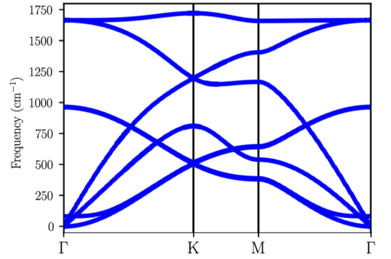
In strong contrast to photons (for which the dispersion relation is fairly simple: $\omega= c k$ ), phonons feature a more complex (solid-dependent) dispersion relation. The figure on the left shows the phonon band-structure (i.e., dispersion) in bilayer graphene (calculated by Lamparski for his thesis in Meunier’s group). Clearly, there is no simple mathematical formula to relate $\omega$ and $k$ . To address this, we will examine two main approximations. Before we move on, a note must be made regarding notations: conventions dictate the momentum for phonons is designated with the letter $q$ , rather than with the letter $k$ as we do with light or with electrons. Do not worry about it too much!

Einstein approximation: In this model, each vibrational mode of the solid is modeled as having the same frequency $\omega_{\rm E}$ , chosen to be the average frequency of the actual set of frequencies. This looks like a crude approximation but the results obtained with it are actually instructive!

Because the phonons are independent, the partition function of the $3N$ vibrations is simply:

$Z=\prod_{k=1}^{3 N} Z_{k},$

where

$Z_{k}=\sum_{n=0}^{\infty} e ^{-\left(n+\frac{1}{2}\right) \hbar \omega_{ E } \beta}=\frac{ e ^{-\frac{1}{2} \hbar \omega_{ E } \beta}}{1- e ^{-\hbar \omega_{ E } \beta}}$

is the partition function for a system with a single frequency. The sum comes from the fact that different modes can be populated with a larger and larger number of quanta of vibrations (just like we did for the simple harmonic oscillator!).

We can thus calculate the internal energy (per mole) using equations we found in Lecture 12: The partition function:

$U=-\left(\frac{\partial \ln Z}{\partial \beta}\right)=3 R \Theta_{ E }\left[\frac{1}{2}+\frac{1}{ e ^{\Theta_{ E } / T}-1}\right]$

where we have introduced the Einstein temperature $\Theta_{ E }=\hbar\omega_E/k_B$ . This equation tends to the equipartition result at high temperature (this is, frankly, quite reassuring but not surprising).

The heat capacity is:

$C=\left(\frac{\partial U}{\partial T}\right)= 3 R \Theta_{ E } \frac{-1}{\left( e ^{\Theta_{ E } / T}-1\right)^{2}} e ^{\Theta_{ E } / T}\left[-\frac{\Theta_{ E }}{T^{2}}\right].$

At the limit of very high temperature, we recover the Dulong-Petit result. At low temperature, we find that the heat capacity falls off very fast (in fact, too fast compared to experiment – see below).
Debye approximation: In this model, we approximate the dispersion relation as

$\omega=v_{ s } q,$

that is: all phonons travel with the same velocity $v_s$ . This is the sound velocity of the mode (in fact, this model is quite good for the so-called acoustic modes, those modes that carry sound in a solid). The maximal frequency is called the Debye frequency $\omega_{ D }=\left(\frac{6 N \pi^{2} v_{ s }^{3}}{V}\right)^{1 / 3}$ and is chosen so that the total number of modes integrates to $3N$ . We define the Debye temperature as $\Theta_{ D }=\frac{\hbar \omega_{ D }}{k_{ B }}$ (this can be seen as a simple change of units between temperature and frequency using two constants: the Planck and Boltzmann constants).

After some calculations, we find that the internal energy is:

$U=\frac{9}{8} N \hbar \omega_{ D }+\frac{9 N \hbar}{\omega_{ D }^{3}} \int_{0}^{\omega_{ D }} \frac{\omega^{3} d \omega}{ e ^{\hbar \omega \beta}-1},$

and the heat capacity (per mole) is:

$C=\frac{9 R}{x_{ D }^{3}} \int_{0}^{x_{ D }} \frac{x^{4} e ^{x} d x}{\left( e ^{x}-1\right)^{2}} \quad {\rm with}\quad x=\hbar \beta \omega.$

Again, the Debye model matches the Dulong-Petit (equipartition) result at high temperature. This is not surprising since we made sure to include the correct number of degrees of freedom (i.e., modes) in the treatment. Even though the frequency values are approximated, we remember that for the equipartition theorem, only the number of modes matters!

The behavior at low temperature is markedly different than Einstein’s result. In fact, the Debye result is much closer to experiment: this makes sense since at low temperature, only the acoustic modes are excited and those are well represented by Debye’s model:

$C_D({\rm low-T})=3 R \times \frac{4 \pi^{4}}{5}\left(\frac{T}{\Theta_{ D }}\right)^{3}.$

We conclude that Einstein is a good approximation for optical modes and Debye is better for acoustic modes (at low-T). The blue box below provides an quick overview of what an optical mode is.

Acoustic and Optical modes

There are two main types of vibrations in a solid. (1) Those that “start at zero”: these are the acoustic modes and (2) those that do not start at zero and have a flatter appearance. The acoustic modes correspond to the transport of sound in the solid. The optical modes got their names from the fact they can be excited with light (or an electromagnetic-wave in general). The reason for this is that an optical mode presents a variation in electrical dipole moment, which, in turn, couples with the electric field of the electromagnetic excitation.

Because a picture is often worth a thousand words, look at the small animation below from physics-animations.com to check the difference:

One thing to remember is that while all structures feature acoustic modes, you need at least two atoms per unit cell to have an optical mode. This is logical: you can’t create a net dipole moment with a single atom!

Note

Comment on tricks of the trade

Physics is sometimes scary because it seems to be leaning heavily on a strong knowledge of mathematics. Since the latter is already hard enough on its own right, people get intimidated with pursuing physics! However, it does not have to be so. Thermodynamics is a tough subject as it requires knowledge in many fields such as quantum mechanics and electro-magnetic theory!

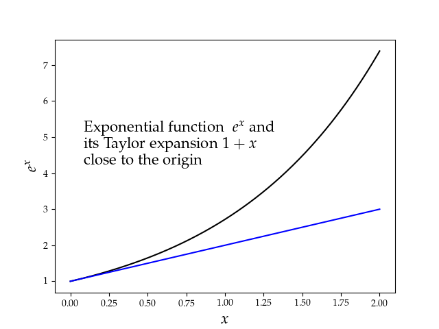
One thing I find useful is to rely on a book of tricks and a future version of this site will have a special book of tricks section included somewhere. Among those tricks, it is good to rely on some useful identities:

$e^{x} \approx 1+x$

$\sin(x) \approx x$

$\sqrt (1+x) \approx 1+\frac{x}{2}$

in all cases, for small enough $x$ . One trick is to remember the plot of those functions where the approximation, as shown in the figure. Another trick to make sense of trigonometry and complex number is to remember the unit circle. This is just a preview of a more substantial page to be available soon!

Key Definitions

Note

Phonon:: A phonon is a collective excitation in a periodic, elastic arrangement of particles in condensed matter. These phonons behave like particles and are often called quasi-particles.

A full list of terms, including the ones provided here, can be found in the Index.

Learning Material

Copy of Slides

The slides for Lecture 16 are available in pdf format here: pdf

Screencast

Test your knowledge

What is a phonon?
1. It is a fundamental quantized elementary vibration of a material.
2. It is a quantum of phony physics.
3. It is a quantum of light.
4. It is a certain type of fermion
What is a dispersion relation?
1. It is a measure on how fast gas molecules travel during a Joule expansion experiment.
2. It is a relation providing a link between the partition function and the temperature.
3. It is a function that provides a relationship between a momentum and a frequency.
4. It is a way to quantize vibrations as a function of the volume of the material.
The Debye and Einstein models provide a description of the heat capacity of a collection of harmonic oscillators. What best describes those models?
1. Debye’s model is superior to Einstein’s at low temperature as it provides an accurate description of the speed of sound in the material.
2. Einstein’s model is always superior to Debye’s at high temperature.
3. Debye’s model is built on the use of an average frequency to describe the system of phonons.
4. Einstein’s model allows for an evaluation of the maximal frequency of the collection of phonons.
In the Einstein model for the harmonic vibrations in a crystal, we define the Einstein temperature as:
1. The temperature at which the effects of special relativity start to influence the vibrational frequencies.
2. The temperature at which the crystal freezes.
3. The temperature where the Brownian motion of the atomic species is most pronounced.
4. The average temperature of the phonons, treated so that the phonon density of states is approximated by a Dirac delta distribution.

Hint

Find the answer keys on this page: Answers to selected test your knowledge questions. Don’t cheat! Try solving the problems on your own first!

Homework Assignment

Solve the following problems from the textbook: