Complement 3: Integral Appendix
Note
This content was crafted by Mr. Ben Madnick.
Note
This integral appendix is modeled after the one in the Blundell and Blundell textbook. An integral appendix is useful in thermodynamics and statistical mechanics because once you are at the thermodynamic limit, distribution functions and probabilities are used to describe various properties of the particles you are studying. These functions are also useful in quantum mechanics, because probabilities and distribution functions become necessary in the regime where classical mechanics fails. One thing worth noting, is that this appendix is here so that, as physicists, we recognize the functions/integrals and use them to simplify otherwise intimidating integrals. For a greater understanding of the derivations of each of the following functions, Introduction to Complex Variables (MATH 4300) is the class to take.
The Gaussian
The Gaussian function ( ) turns up in many statistical problems. It is
also called the normal distribution or bell curve. The Gaussian
is a function of the form
) turns up in many statistical problems. It is
also called the normal distribution or bell curve. The Gaussian
is a function of the form  where
where  is a constant. When plotted, as in Figure 1, you can see
the bell curve.
is a constant. When plotted, as in Figure 1, you can see
the bell curve.
Figure 1
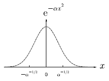
The Gaussian bell function .
From Figure 1, we can see that the function is at a maximum
when  . Now since we have described the Gaussian, we can
discuss integrating it. We will evaluate using a two-dimensional
integral
. Now since we have described the Gaussian, we can
discuss integrating it. We will evaluate using a two-dimensional
integral

Here  is our desired integral. We can evaluate the left side using polar coordinates:

Therefore:

Making the substitution:

This now becomes a simple integral:

which can be computed so that:

Differentiating both sides with respect to we find a
general formula

Since all of these functions are even, these integrals from
 is just half of this result. This is where
they become useful in physics, as this is the velocity distribution for
the motion of gas molecules. But what about if
is just half of this result. This is where
they become useful in physics, as this is the velocity distribution for
the motion of gas molecules. But what about if  is raised to an
odd power? Since the function would be odd, integrating across symmetric
bounds means the integral is 0. But that means we still have to consider
the integration space from
is raised to an
odd power? Since the function would be odd, integrating across symmetric
bounds means the integral is 0. But that means we still have to consider
the integration space from

Making the substitution:

From here we have a general formula for when is raised to an
odd power. The general formula is

The factorial integral and the Gamma Function
Once the class shifts more to the statistical mechanics portion, thermodynamic behavior is studied using mathematical functions and the partition function. The Gamma Function is a useful tool, and an important function to recognize. It’s derivation and use can also be studied in Introduction to Complex Variables. The factorial integral is useful, because once recognized, it simplifies many of the later integrals covered in this appendix and course. The factorial integral is

It may not be noticed initially, but this function allows one to define the factorial for a non-integer number. Here is where the Gamma Function truly becomes a useful mathematical tool. The traditional definition of the Gamma Function is

When plotted, the Gamma function looks like Figure 2.
Figure 2
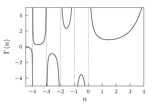
The Gamma Function  showing the singularities for integer values of
  . For positive, integer
  ,
, 
Riemann Zeta Function
Another function that is involved in many useful integrals is the Riemann zeta function. The Riemann zeta function is defined by
When plotted, the Riemann zeta function appears as

Figure 3
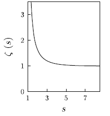
The Riemann zeta function for values 
Note that the series diverges when  . The analysis of this
series can be studied more in Introduction to Complex Variables, but in
this class we are interested in its appearance in integrals such as the
Bose Integral. The Bose Integral is, as implied from the name,
useful in quantum mechanics and statistical mechanics for studying boson
gases such as photons. The Bose integral will appear as a consequence of
density of states and symmetric states of bosons, but that derivation
will be covered in later lectures. The Bose Integral is defined by
. The analysis of this
series can be studied more in Introduction to Complex Variables, but in
this class we are interested in its appearance in integrals such as the
Bose Integral. The Bose Integral is, as implied from the name,
useful in quantum mechanics and statistical mechanics for studying boson
gases such as photons. The Bose integral will appear as a consequence of
density of states and symmetric states of bosons, but that derivation
will be covered in later lectures. The Bose Integral is defined by

Evaluating this. We multiply by a factor of 1, in this case, 

The next two steps of this evaluation are explained in greater detail in a complex analysis class. They involve geometric series of complex exponential functions. If you are interested in mathematical functions, it is a good class to take:

Thus we have that the Bose integral is

Similarly, we also have that

The Polylogarithm
The Polylogarithm function,  is used in the
evaluation of Bose-Einstein and Fermi-Dirac distributions. These
distribution functions become important when we begin discussing bosons
and fermions. The polylogarithm is defined as
is used in the
evaluation of Bose-Einstein and Fermi-Dirac distributions. These
distribution functions become important when we begin discussing bosons
and fermions. The polylogarithm is defined as

Before we begin showing how this function is useful in solving the distribution functions, we should note that we can write the following geometric progression

we then have this integral

Making the substitution

Therefore

So the integral becomes

This integral should look familiar as it is the Gamma function

Making the substitution  also yields a familiar looking function

So we know that this solves the Fermi-Dirac distribution, but what about the Bose-Einstein distribution? The short answer is that it does. If you repeat the preceding process for the BE distribution you will find

Combining the two equations we write in general that

Performing just a little bit more analysis on the polylogarithm shows
that when  we have that

Also we can note that

The Dirac Delta function
Here we are going to discuss arguably the simplest function in this appendix. Technically it is a distribution or generalized function. The Dirac delta function is an infinitely high, infinitesimally narrow spike at the origin with an area of 1.

and

This can be visualized in Figure 4.
Figure 4
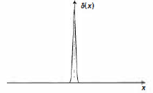
The Dirac delta function, except imagine the curve as an infinitely high and infinitesimally narrow spike
This function has some interested properties. What if we want to shift
the spike to some arbitrary value  ?. We therefore would have
that
?. We therefore would have
that

and

What if the Dirac delta is multiplied by a continuous function
 ? We would therefore have

and

Imagine that the delta function isolates the value of  and
the integral collapses onto that point. The Dirac delta makes many
integral simple to evaluate. However, don’t just throw it in to any
integral in order to simplify it.
and
the integral collapses onto that point. The Dirac delta makes many
integral simple to evaluate. However, don’t just throw it in to any
integral in order to simplify it.
Fourier transforms
While possibly briefly covered in Quantum Physics I and Quantum Physics II, this appendix is here to hopefully give a more thorough explanation of its importance in physics. The Fourier transform allows one to “switch” between time space and frequency space. It is useful for the studying of waves and heat flow problems, which are covered more in a differential equations course. The Fourier transform is defined by

This converts the function from a function of time to a
function of frequency. To inverse the transform, we use an inverse
transform defined as:

One thing to note, be careful about the exponential term. Remember for
which transform the exponential term is positive and negative. Both are
imaginary but the sign changes between transforms. Also to convert to
frequency space the factor of  is important and
not to be left behind, to ensure proper normalization.
is important and
not to be left behind, to ensure proper normalization.
Conclusion
Hopefully this appendix becomes will prove a useful tool not just for Thermodynamics and Statistical Mechanics, but for other math and physics courses. Many of the functions covered in this appendix will also be seen in Astrophysics, Introductory Quantum Mechanics, Complex Variables, and other 4000 level courses at RPI.